In this blog, I will introduce several classic cnn frameworks, including VGG, googleNet, resNet, DenseNet, each one with a absolute new perspective, greatly promotes the development of computer vision.

1. LeNet-5

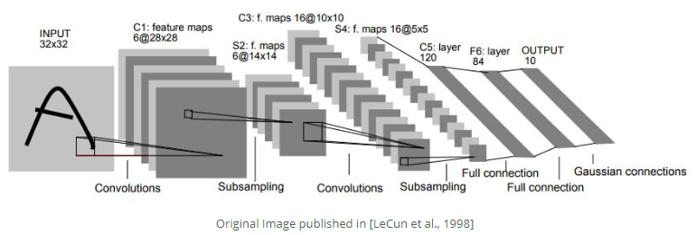
LeNet-5, a classical convolutional neural network that was introduced back to 1998, is aimed to recognize the digits from 0-9. The first figure below is the model architecture form the paper and the second one is the figure that is similar to figure 1. LeNet-5 is such a classical model that it consists of two convolution layers followed be average pooling layers for each and apply three fully connected layers in the end of the network. The second model is quite similar to LeNet-5 except using max pooling layers.

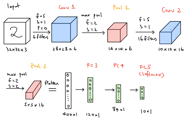
As shown above fot the LeNet-5 modified model, the network takes a image as the input and convolve it with 6 filters and stride of 1, which results in a output and then apply the output to a max pooling layer with the filter size of and stride of , which leads to a output. Then apply the same convolution and max pooling layer again to obtain a output. At the end of the network , the output is flattend to a vector with the size and then apply two fully connected layers to it anf finally achieve the estimated output with the size of by using softmax.

Take the second architecture as an example, let’s practice how to compute the amounts of the parameters that are needed to learn in each layer of the network.

Layers	Activation Size	Number of Parameters
		0
		0
		0

Where is the kernel_size, is the stride, is the padding, is the number of kernels, is the bias. In the netowrk, they applied the non-linearity function sigmoid after each max pooling layer. In summary, the total number of of parameters that the network needs to learn is approximately 65000. According to this classical architecture, there are actually several patterns that the modern architectures still apply, which are the general structures of the networks, $Conv->Pool->Conv->Pool->Fc->Fc$. That is, convolution layers are followed by pooling layers and a few of fully connected layers are located in the end of the metwork. Additionally, the trends of nowadays networks that and decrease while increases as the networks go deeper are still applying.
Below are codes of LeNet-5 implemented by pytoch

import torch.nn as nn
import torch

class LeNet(nn.Module):
    """This class implements the classical LeNet-5 network"""
    def __init__(self, in_clannels, out_channels) -> None:
        super().__init__()
        #Here we need to specify the size of the input as 32 * 32 *3
        self.nn = nn.Sequential(
            nn.Conv2d(1, 6, kernel_size = 5, stride = 1, padding = 0),
            nn.Sigmoid(),
            nn.MaxPool2d(kernel_size = 2, stride = 2),
            nn.Conv2d(6, 16, 5, 1),
            nn.Sigmoid(),
            nn.MaxPool2d(kernel_size = 2, stride = 2),
            nn.Flatten(),
            nn.Linear(400, 120),
            nn.Sigmoid(),
            nn.Linear(120, 84),
            nn.Sigmoid(),
            nn.Linear(84, out_channels),
            nn.Softmax() # Here we need to notice that Softmax is neccssary
        )
    def forward(self, x):
        return self.nn(x)

        

2. AlexNet

AlexNet, intriduced in 2012, employs an 8-layer convolutional neural network where the architecture is quite similar to LeNet-5, but there are also some significant differences. First, AlexNet is much deeper since it consists of finve convolution layers, two hidden fully-connected layers and one onle fully-connected output layer as shown in the figure below. Aside from that, AlexNet used the ReLU activation function instead of Sigmoid and the ReLu function is processed after each convolution layer. Futhermore, dropout is also used after each fully connected layer except the output layer.

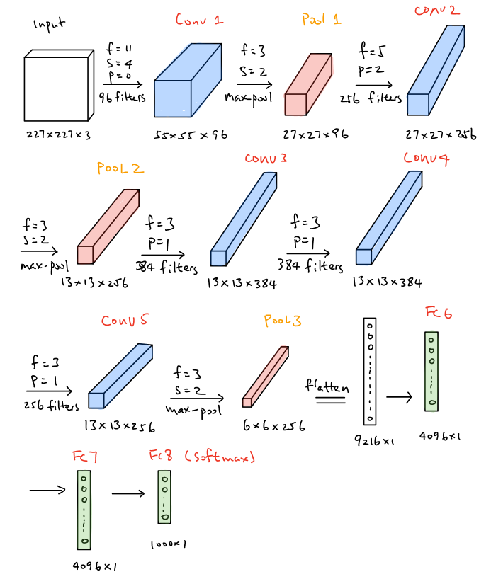
In the first layer of Alexnet, the convolution filter size is . This is because this model is implemented to classify the inputs from ImageNet, the dataset which has bigger size. Consequently, a larger convolution window is applied in the first layer in order to capture the object. The brief structure of AlexNet can eb illustrated as . Notice that all the convolutional layers in ALexNet apply the same padding and as the network goes deeper, more filters are used to convolve while the height and width of the activation shape are similar. Futhermore, dropout is used after each layer in order to address the overfitting.
The amounts of the parameters that are needed to learn in each layer of the network is demonstrated below.

Layers	Activation Size	Number of Parameters
		0
		0
		0
		0

The total number of parameters needed to learn in AlexNet is approximately 60 million, which are way larger than LeNet-5 are. The pytorch version code of AlexNet is illustrated below

import torch.nn as nn
import torch

class AlexNet(nn.Module):
    """This class implements the classical AlexNet network"""
    def __init__(self, in_clannels, out_channels) -> None:
        super().__init__()
        #Here we need to specify the size of the input as 32 * 32 *3
        self.nn = nn.Sequential(
            nn.Conv2d(in_channels, 96, kernel_szie = 11, stride = 4, padding  = 1),
            nn.ReLU(),
            nn.MaxPool2d(kernel_size = 3, stride = 2),
            nn.Conv2d(96, 256, kernel_szie = 5, stride = 1, padding  = 2),
            nn.ReLU(),
            nn.MaxPool2d(kernel_size = 3, stride = 2),
            nn.Conv2d(256, 384, kernel_szie = 3, stride = 1, padding  = 1),
            nn.ReLU(),
            nn.Conv2d(384, 384, kernel_szie = 3, stride = 1, padding  = 1),
            nn.ReLU(),
            nn.Conv2d(384, 256, kernel_szie = 3, stride = 1, padding  = 1),
            nn.ReLU(),
            nn.MaxPool2d(kernel_size = 3, stride = 2),
            nn.Flatten(),
            nn.Linear(6400, 4096),
            nn.ReLU(),
            nn.Dropout(p = 0.5),
            nn.Linear(4096, 4096),
            nn.ReLU(),
            nn.Dropout(p = 0.5),
            nn.Linear(4096, 1000),
            nn.Softmax()
        )
    def forward(self, x):
        return self.nn(x)

3. VGG-16

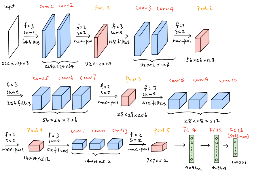
VGG-16, introduced in 2014, employs a 16-layer network, which is much deeper than ALexNet but offers a simpler network by replacing large kernel size filters withi multiple 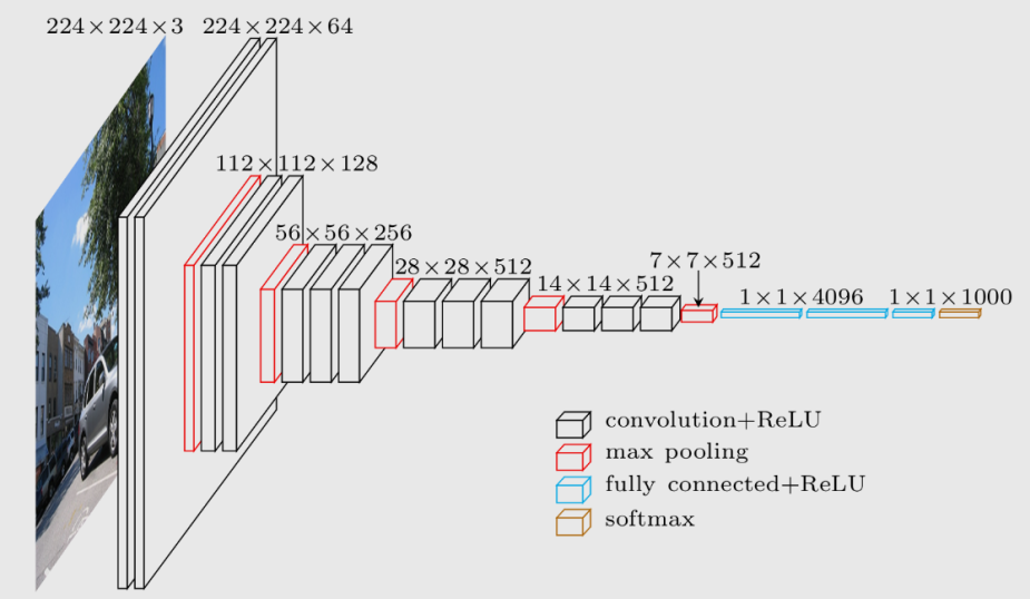kernel-sized filters one after another. Aside from that, VGG-16 focuses on the possily simpler network where all the convolutional layer’s filter size are with stride of 1 and same padding whereas the mas pooling layers al apply filter and stride of . The brief summary of VGG-16 is illustrated below

The patterns of VGG-16 are quite uniform that the network takes image as the input, followed by a stack of two and three convolutional layers and Relu activation function, then reduce the height anf width by using pooling layer. For the number of filters in each convolutional layer, they are , where as the network goes deeper the number of filters double in each stack of convolutional layer. Overall, there are approximately 138 million parameters needed to learn. Another phenomenon that the modern networks also apply is that as the network goes deeper, , decrease due to the pooling layers and increases due to the increasing number of filters in convolutional layers.

The pytorch version of VGG-16 is illustrated as follow

from sympy import Mul
import torch.nn as nn
import torch

class VGG_16(nn.Module):
    """This class implements the classical LeNet-5 network"""
    def __init__(self, in_clannels, out_channels) -> None:
        super().__init__()
        #Here we need to specify the size of the input as 32 * 32 *3
        self.nn = nn.Sequential(
            MultiConv(in_clannels, 64, 2),
            MultiConv(64, 128, 2),
            MultiConv(128, 256, 3),
            MultiConv(256, 512, 3),
            MultiConv(512, 512, 3),
            nn.Flatten(),
            nn.Linear(7*7*512, 4096),
            nn.ReLU(inplace = True),
            nn.Dropout(p = 0.5),
            nn.Linear(4096, 4096),
            nn.ReLU(inplace = True),
            nn.Dropout(p = 0.5),
            nn.Linear(4096, out_channels),
            nn.Softmax()
        )
    def forward(self, x):
        return self.nn(x)


class MultiConv(nn.Module):
    """This class implements double conv operation"""
    def __init__(self, in_channels, out_channels, num_conv) -> None:
        super().__init__()
        multi_Conv = [nn.Conv2d(out_channels, out_channels, kernel_size = 3, stride = 1, padding = 1)] * (num_conv - 1)
        self.multiConv = nn.Sequential(
            nn.Conv2d(in_channels, out_channels, kernel_size = 3, padding = 1, stride = 1),
            *multi_Conv,
            nn.ReLU(inplace = True),
            nn.MaxPool2d(kernel_size = 2, stride = 2)
        )
    
    def forward(self, x):
        return self.nn(x)


if __name__ == "__main__":
    model = VGG_16(1, 1000)
    print(model)
        

4.GoogleNet

The inception Network was one of the major breakthroughs in the fields Neural metowrks, particularly for CNNs, So far there are three versions of inception Networks, which are named Inception version 1,2 and 3. The first version entered the field in 2014. and as the name “GoogleNet” suggests, it was developed by a team at google. This network was responsible for setting state of art for classification and detection in the ILSVRC. The first version of the Inception networks is referred to as GoogleNet.

if a network is built with many deep layers it might face the problem of overfitting. To solve this problem, the authors in the research paper Going deeper with convolutions proposed the GoogleNet architecture with the idea of having filters with multiple sizes that can operate on the same level. With this idea, the network actually becomes wider ranther deeper. Below is an image showing a Naive inception Module.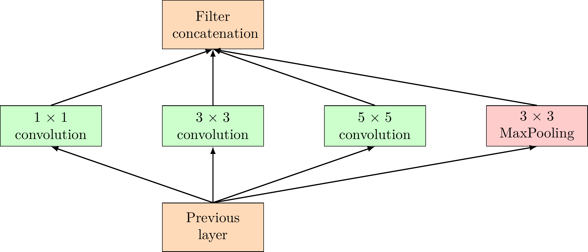

As can be seen in the above diagram, the convolution operation is performed on inputs with three filter sizes: and . A max-pooling operation is also perfoemed with the convolutions and is then sent into the next inception module.
Since neural networks are time-consuming and expensive to train, the authors limit the number of input channels by adding an extra 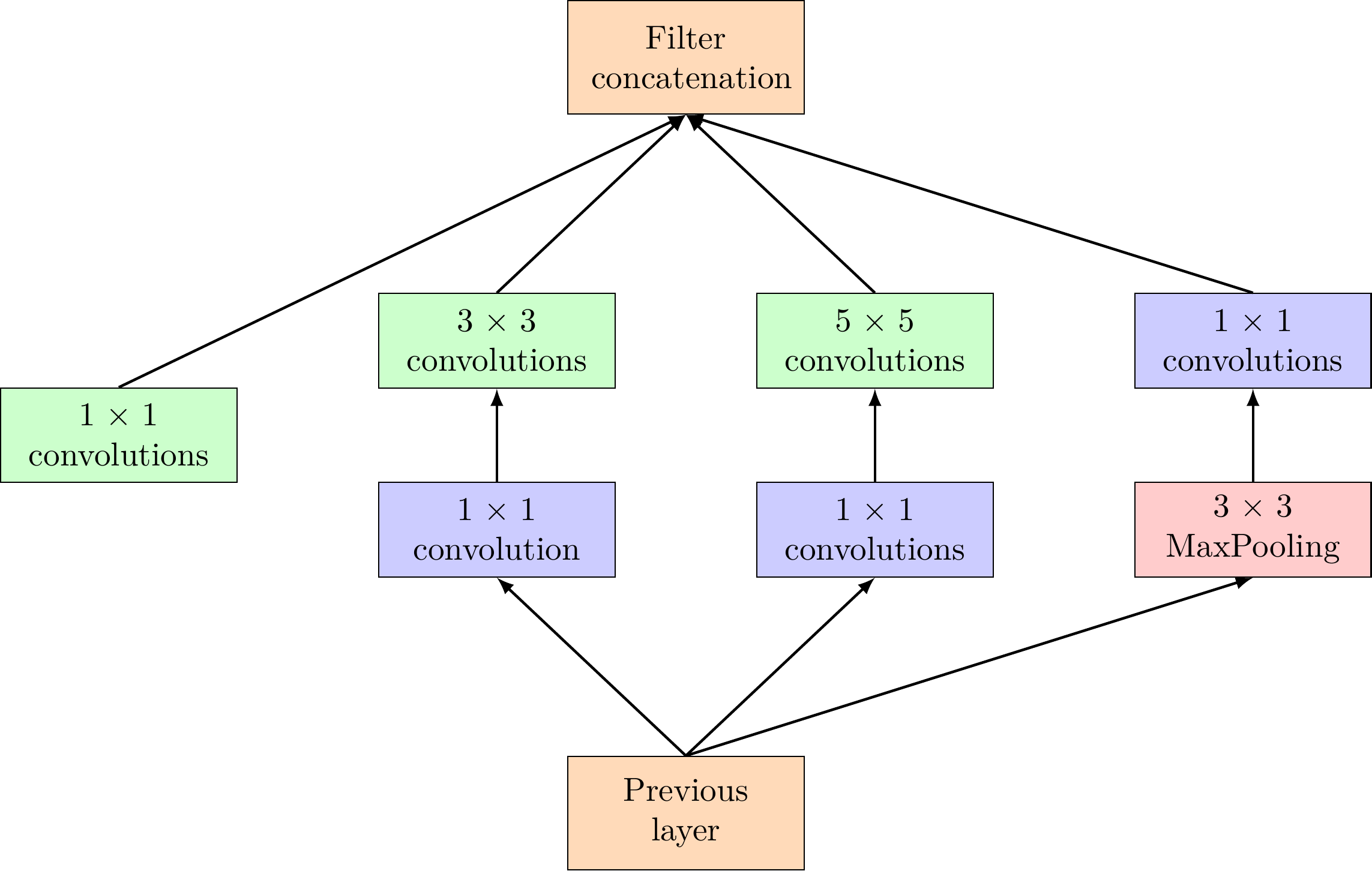convolution before the and covolutions to reduce the dimensions of the network and perform faster computations. Below is an image showing a Naive Inception Module with this addition.

These are the building blocks of GoogleNet. Below is a detailed report on its architecture.

GoogleNet Architecture

The GoogleNet architecture is 22 layers deep, with 27 pooling layers included. There are a 9 inception modules stacked linearly in total. The ends of the inception modules are connected to the global average pooling layer. Below is a zoomed-out image of the full GoogleNet architecture.

The pytorch version of googleNet is illustrated as below

from sympy import true
import torch 
import torch.nn as nn 




class BasicConv2d(nn.Module):
    """This class implements basic conv2d operations"""
    def __init__(self, in_channels, out_channels, *args) -> None:
        super().__init__()
        self.nn = nn.Sequential(
            nn.Conv2d(in_channels, out_channels, *args),
            nn.ReLU(inplace = True)
        )
    
    def forward(self, x):
        return self.nn(x)

class InceptionAux(nn.Module):
    """This class implements the inception module in the googleNet infrastructure"""
    def __init__(self, in_channels, num_classes) -> None:
        super().__init__()
        self.inceptionaux = nn.Sequential(
            nn.AvgPool2d(kernel_size = 5, stride = 3),
            BasicConv2d(in_channels, 128, kernel_size = 1),
            nn.Flatten(),
            nn.Linear(2048, 1024),
            nn.ReLU(inplace = True),
            nn.Dropout(p = 0.5),
            nn.Linear(1024, num_classes),
            nn.Softmax()
        )
    
    def forward(self, x):
        return self.inceptionaux(x)

class Inception(nn.Module):
    """This class implements inception module"""
    def __init__(self, in_channels, ch1x1, ch3x3red, ch3x3, ch5x5red, ch5x5, pool_proj) -> None:
        super().__init__()
        self.branch1 = BasicConv2d(in_channels, ch1x1, kerner_size = 1)
        self.branch2 = nn.Sequential(
            BasicConv2d(in_channels, ch3x3red, kernel_size = 1),
            BasicConv2d(ch3x3red, ch3x3, kernel_size = 3, padding = 1)
            )
        self.branch3 = nn.Sequential(
            BasicConv2d(in_channels, ch5x5red, kernel_size = 1),
            BasicConv2d(ch5x5red, ch5x5, kernel_size = 5, padding = 2)
        )

        self.branch4 = nn.Sequential(
            nn.MaxPool2d(kernel_size = 3, padding = 1, stride = 1),
            BasicConv2d(in_channels, pool_proj, kernel_size = 1)
        )
    
    def forward(self, x):
        branch1 = self.branch1(x)
        branch2 = self.branch2(x)
        branch3 = self.branch3(x)
        branch4 = self.branch4(x)
        return torch.cat([branch1, branch2, branch3, branch4], dim = 1)

class GoogLeNet(nn.Module):
    def __init__(self, num_classes=1000, aux_logits=True, init_weights=False):
        super(GoogLeNet, self).__init__()
        self.aux_logits = aux_logits

        self.conv1 = BasicConv2d(3, 64, kernel_size=7, stride=2, padding=3)
        self.maxpool1 = nn.MaxPool2d(3, stride=2, ceil_mode=True)

        self.conv2 = BasicConv2d(64, 64, kernel_size=1)
        self.conv3 = BasicConv2d(64, 192, kernel_size=3, padding=1)
        self.maxpool2 = nn.MaxPool2d(3, stride=2, ceil_mode=True)

        self.inception3a = Inception(192, 64, 96, 128, 16, 32, 32)
        self.inception3b = Inception(256, 128, 128, 192, 32, 96, 64)
        self.maxpool3 = nn.MaxPool2d(3, stride=2, ceil_mode=True)

        self.inception4a = Inception(480, 192, 96, 208, 16, 48, 64)
        self.inception4b = Inception(512, 160, 112, 224, 24, 64, 64)
        self.inception4c = Inception(512, 128, 128, 256, 24, 64, 64)
        self.inception4d = Inception(512, 112, 144, 288, 32, 64, 64)
        self.inception4e = Inception(528, 256, 160, 320, 32, 128, 128)
        self.maxpool4 = nn.MaxPool2d(3, stride=2, ceil_mode=True)

        self.inception5a = Inception(832, 256, 160, 320, 32, 128, 128)
        self.inception5b = Inception(832, 384, 192, 384, 48, 128, 128)

        if self.aux_logits:
            self.aux1 = InceptionAux(512, num_classes)
            self.aux2 = InceptionAux(528, num_classes)

        self.avgpool = nn.AdaptiveAvgPool2d((1, 1))
        self.dropout = nn.Dropout(0.4)
        self.fc = nn.Linear(1024, num_classes)
        if init_weights:
            self._initialize_weights()

    def forward(self, x):
        # N x 3 x 224 x 224
        x = self.conv1(x)
        # N x 64 x 112 x 112
        x = self.maxpool1(x)
        # N x 64 x 56 x 56
        x = self.conv2(x)
        # N x 64 x 56 x 56
        x = self.conv3(x)
        # N x 192 x 56 x 56
        x = self.maxpool2(x)

        # N x 192 x 28 x 28
        x = self.inception3a(x)
        # N x 256 x 28 x 28
        x = self.inception3b(x)
        # N x 480 x 28 x 28
        x = self.maxpool3(x)
        # N x 480 x 14 x 14
        x = self.inception4a(x)
        # N x 512 x 14 x 14
        if self.training and self.aux_logits:    # eval model lose this layer
            aux1 = self.aux1(x)

        x = self.inception4b(x)
        # N x 512 x 14 x 14
        x = self.inception4c(x)
        # N x 512 x 14 x 14
        x = self.inception4d(x)
        # N x 528 x 14 x 14
        if self.training and self.aux_logits:    # eval model lose this layer
            aux2 = self.aux2(x)

        x = self.inception4e(x)
        # N x 832 x 14 x 14
        x = self.maxpool4(x)
        # N x 832 x 7 x 7
        x = self.inception5a(x)
        # N x 832 x 7 x 7
        x = self.inception5b(x)
        # N x 1024 x 7 x 7

        x = self.avgpool(x)
        # N x 1024 x 1 x 1
        x = torch.flatten(x, 1)
        # N x 1024
        x = self.dropout(x)
        x = self.fc(x)
        # N x 1000 (num_classes)
        if self.training and self.aux_logits:   # eval model lose this layer
            return x, aux2, aux1
        return x

    def _initialize_weights(self):
        for m in self.modules():
            if isinstance(m, nn.Conv2d):
                nn.init.kaiming_normal_(m.weight, mode='fan_out', nonlinearity='relu')
                if m.bias is not None:
                    nn.init.constant_(m.bias, 0)
            elif isinstance(m, nn.Linear):
                nn.init.normal_(m.weight, 0, 0.01)
                nn.init.constant_(m.bias, 0)

The detailed architecture and parameters are explained in the image below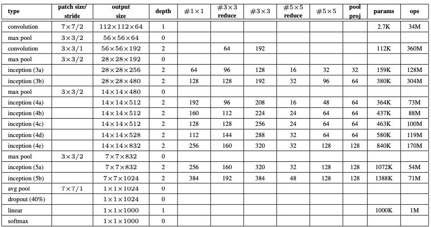

ResNets

After the first CNN-based architecture (AlexNet) that win the ImageNet 2012 competition, every subsequent winning architecture use more layers in a deep neural network to reduce the error rate. This works for less number of layers, but when we increase the number of layers, there is a common problem in deep learning associated with that called Vanishing/Exploding gradient. This causes the gradient to become 0 or too large. Thus when we increases number of layers, the training and test error rate also increases.

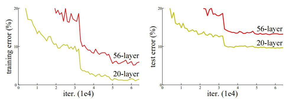
In the above plot, we can observe that a 56-layer CNN gives more error rate on both training and testing dataset than a 20-layer CNN architecture, if this was the result over fitting, then we should have lower traing error in 56-layer CNN but then it also has higher training error. After analyzing more on error rate the authors were able to reach conclusion that it is caused by vanishing /exploding gradient.
ResNet, which was proposed in 2015 by reseraches at Microsoft Research introduced a new architecture called Residual Network.

Residual Block:
In order to solve the problem of the vanishing/exploding gradient, this architecture introduced the concept called Residual Network. In this network we use a technique called skip connections. The skip connection skips training from a few layers and connects directly to the output.
The approach behind this network is instead of layers learn the underlying mapping, we allow network fit the residual mapping. So, instead of say 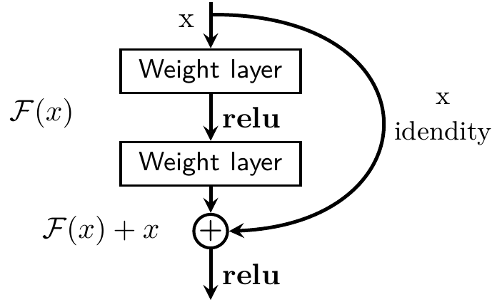, initial mapping, let the network fit, which gives .

The advantage of adding this type of skip connection is because if any layer hurt the performance of architecture then it will be skipped by regularization. So, this results in training very deep neural network without the problems caused by vanishing /exploding gradient. The authors of the paper experimented on 100-1000 layers on CIFAR-10 dataset. There is similar approach called “highway networks”, these networks also uses skip connection. Similar to LST< these skip connections also uses parametric gates. These gates determine how much information passes through the skip connection. This architecture however has not provide accuracy better than ResNet architecture.

Network Architecture

This network uses a 34-layer plain network architecture inspired by VGG-19 in which then the shortcut connection is added. These shortcut connections then convert the architecture into residual network.

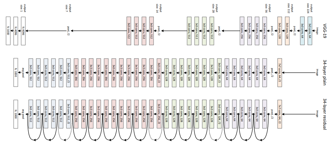
Here I do not provide the pytorch version of this kind work since it is very easy to implement under python.